
Coffee Ratings
TidyTuesday project modelling coffee ratings

Intro
Today I am going to explore Coffee Ratings for this week’s Tidy Tuesday challenge. The data comes from the Coffee Quality Database. The great thing about Tidy Tuesday is that we can do whatever we want with the data. There are no rules or directions!
This data is very interesting with many features and looks ripe for a predictive model. I can use the various ratings provided to predict either a quantitative method, like what the ‘total_cup_score’ (Overall rating) is, or a qualitative measure, like what species of bean (Arabica or Robusta) or perhaps the country of origin.
Predicting scores strikes me as a classic regression problem, best tackled by linear models or random forests, and classification could be solved with logistic regression, Naive Bayes, SVM or even neural networks. I’ve NEVER used tidymodels before, so let’s give it a go, make some mistakes, and see what we can learn.
But first, some brief background of our data from the TidyTuesday repo:
There is data for both Arabica and Robusta beans, across many countries and professionally rated on a 0-100 scale. All sorts of scoring/ratings for things like acidity, sweetness, fragrance, balance, etc - may be useful for either separating into visualizations/categories or for modeling/recommenders.
Wikipedia on Coffee Beans:
The two most economically important varieties of coffee plant are the Arabica and the Robusta; ~60% of the coffee produced worldwide is Arabica and ~40% is Robusta. Arabica beans consist of 0.8–1.4% caffeine and Robusta beans consist of 1.7–4% caffeine.
Setup
library(tidytuesdayR)
library(tidyverse)
## ── Attaching packages ──────────────────── tidyverse 1.3.0 ──## ✓ ggplot2 3.3.2 ✓ purrr 0.3.4
## ✓ tibble 3.0.1 ✓ dplyr 1.0.0
## ✓ tidyr 1.1.0 ✓ stringr 1.4.0
## ✓ readr 1.3.1 ✓ forcats 0.5.0## ── Conflicts ─────────────────────── tidyverse_conflicts() ──
## x dplyr::filter() masks stats::filter()
## x dplyr::lag() masks stats::lag()library(tidymodels)## ── Attaching packages ─────────────────── tidymodels 0.1.0 ──## ✓ broom 0.5.6 ✓ rsample 0.0.6
## ✓ dials 0.0.6 ✓ tune 0.1.0
## ✓ infer 0.5.1 ✓ workflows 0.1.1
## ✓ parsnip 0.1.1 ✓ yardstick 0.0.6
## ✓ recipes 0.1.12## ── Conflicts ────────────────────── tidymodels_conflicts() ──
## x scales::discard() masks purrr::discard()
## x dplyr::filter() masks stats::filter()
## x recipes::fixed() masks stringr::fixed()
## x dplyr::lag() masks stats::lag()
## x dials::margin() masks ggplot2::margin()
## x yardstick::spec() masks readr::spec()
## x recipes::step() masks stats::step()library(knitr)
library(kableExtra)##
## Attaching package: 'kableExtra'## The following object is masked from 'package:dplyr':
##
## group_rowsknitr::opts_chunk$set(
fig.height = 5,
fig.width = 8,
message = FALSE,
warning = FALSE,
dpi = 180,
include = TRUE
)Load the data
tuesdata <- tidytuesdayR::tt_load(2020, week = 28)
coffee_ratings <- tuesdata$coffee_ratings
EDA
Now that we have our data and let’s dive in. Let’s review the summary statistics with skimr.
coffee_ratings %>%
skimr::skim()| Name | Piped data |
| Number of rows | 1339 |
| Number of columns | 43 |
| _______________________ | |
| Column type frequency: | |
| character | 24 |
| numeric | 19 |
| ________________________ | |
| Group variables | None |
Variable type: character
| skim_variable | n_missing | complete_rate | min | max | empty | n_unique | whitespace |
|---|---|---|---|---|---|---|---|
| species | 0 | 1.00 | 7 | 7 | 0 | 2 | 0 |
| owner | 7 | 0.99 | 3 | 50 | 0 | 315 | 0 |
| country_of_origin | 1 | 1.00 | 4 | 28 | 0 | 36 | 0 |
| farm_name | 359 | 0.73 | 1 | 73 | 0 | 571 | 0 |
| lot_number | 1063 | 0.21 | 1 | 71 | 0 | 227 | 0 |
| mill | 315 | 0.76 | 1 | 77 | 0 | 460 | 0 |
| ico_number | 151 | 0.89 | 1 | 40 | 0 | 847 | 0 |
| company | 209 | 0.84 | 3 | 73 | 0 | 281 | 0 |
| altitude | 226 | 0.83 | 1 | 41 | 0 | 396 | 0 |
| region | 59 | 0.96 | 2 | 76 | 0 | 356 | 0 |
| producer | 231 | 0.83 | 1 | 100 | 0 | 691 | 0 |
| bag_weight | 0 | 1.00 | 1 | 8 | 0 | 56 | 0 |
| in_country_partner | 0 | 1.00 | 7 | 85 | 0 | 27 | 0 |
| harvest_year | 47 | 0.96 | 3 | 24 | 0 | 46 | 0 |
| grading_date | 0 | 1.00 | 13 | 20 | 0 | 567 | 0 |
| owner_1 | 7 | 0.99 | 3 | 50 | 0 | 319 | 0 |
| variety | 226 | 0.83 | 4 | 21 | 0 | 29 | 0 |
| processing_method | 170 | 0.87 | 5 | 25 | 0 | 5 | 0 |
| color | 218 | 0.84 | 4 | 12 | 0 | 4 | 0 |
| expiration | 0 | 1.00 | 13 | 20 | 0 | 566 | 0 |
| certification_body | 0 | 1.00 | 7 | 85 | 0 | 26 | 0 |
| certification_address | 0 | 1.00 | 40 | 40 | 0 | 32 | 0 |
| certification_contact | 0 | 1.00 | 40 | 40 | 0 | 29 | 0 |
| unit_of_measurement | 0 | 1.00 | 1 | 2 | 0 | 2 | 0 |
Variable type: numeric
| skim_variable | n_missing | complete_rate | mean | sd | p0 | p25 | p50 | p75 | p100 | hist |
|---|---|---|---|---|---|---|---|---|---|---|
| total_cup_points | 0 | 1.00 | 82.09 | 3.50 | 0 | 81.08 | 82.50 | 83.67 | 90.58 | ▁▁▁▁▇ |
| number_of_bags | 0 | 1.00 | 154.18 | 129.99 | 0 | 14.00 | 175.00 | 275.00 | 1062.00 | ▇▇▁▁▁ |
| aroma | 0 | 1.00 | 7.57 | 0.38 | 0 | 7.42 | 7.58 | 7.75 | 8.75 | ▁▁▁▁▇ |
| flavor | 0 | 1.00 | 7.52 | 0.40 | 0 | 7.33 | 7.58 | 7.75 | 8.83 | ▁▁▁▁▇ |
| aftertaste | 0 | 1.00 | 7.40 | 0.40 | 0 | 7.25 | 7.42 | 7.58 | 8.67 | ▁▁▁▁▇ |
| acidity | 0 | 1.00 | 7.54 | 0.38 | 0 | 7.33 | 7.58 | 7.75 | 8.75 | ▁▁▁▁▇ |
| body | 0 | 1.00 | 7.52 | 0.37 | 0 | 7.33 | 7.50 | 7.67 | 8.58 | ▁▁▁▁▇ |
| balance | 0 | 1.00 | 7.52 | 0.41 | 0 | 7.33 | 7.50 | 7.75 | 8.75 | ▁▁▁▁▇ |
| uniformity | 0 | 1.00 | 9.83 | 0.55 | 0 | 10.00 | 10.00 | 10.00 | 10.00 | ▁▁▁▁▇ |
| clean_cup | 0 | 1.00 | 9.84 | 0.76 | 0 | 10.00 | 10.00 | 10.00 | 10.00 | ▁▁▁▁▇ |
| sweetness | 0 | 1.00 | 9.86 | 0.62 | 0 | 10.00 | 10.00 | 10.00 | 10.00 | ▁▁▁▁▇ |
| cupper_points | 0 | 1.00 | 7.50 | 0.47 | 0 | 7.25 | 7.50 | 7.75 | 10.00 | ▁▁▁▇▁ |
| moisture | 0 | 1.00 | 0.09 | 0.05 | 0 | 0.09 | 0.11 | 0.12 | 0.28 | ▃▇▅▁▁ |
| category_one_defects | 0 | 1.00 | 0.48 | 2.55 | 0 | 0.00 | 0.00 | 0.00 | 63.00 | ▇▁▁▁▁ |
| quakers | 1 | 1.00 | 0.17 | 0.83 | 0 | 0.00 | 0.00 | 0.00 | 11.00 | ▇▁▁▁▁ |
| category_two_defects | 0 | 1.00 | 3.56 | 5.31 | 0 | 0.00 | 2.00 | 4.00 | 55.00 | ▇▁▁▁▁ |
| altitude_low_meters | 230 | 0.83 | 1750.71 | 8669.44 | 1 | 1100.00 | 1310.64 | 1600.00 | 190164.00 | ▇▁▁▁▁ |
| altitude_high_meters | 230 | 0.83 | 1799.35 | 8668.81 | 1 | 1100.00 | 1350.00 | 1650.00 | 190164.00 | ▇▁▁▁▁ |
| altitude_mean_meters | 230 | 0.83 | 1775.03 | 8668.63 | 1 | 1100.00 | 1310.64 | 1600.00 | 190164.00 | ▇▁▁▁▁ |
Check Initial Assumptions
I originally wanted to predict “total_cup_points”. However, after some review it appears that this field is simply the sum of ten other ratings, from aroma to cupper_points. What I really want to predict is Cupper Points. This is the reviewer’s (aka the Cupper’s) personal overall rating for the cup of joe. I can use this as dependant variable in a regression analysis. This should help me identify which features (aroma, acidity, elevation, country of origin?) influence the final rating the most.
Potential Features
Before we dig further into the data, let’s speculate what might factors go into a superior coffee bean. If coffee is like wine, then perhaps region (lat, long, altitude, preciptation, average hours of sunlight, etc) makes a big difference. Perhaps certain companies utilize best practices and farming techniques. Maybe certain processing methods are better than others. We are given the testing date and the expiration date, so we can add a feature that measures how fresh the beans are. These features and more could be really important or totally useless. I have no idea! Let’s see what the data has to say about it.
The wiki in the readme suggests that coffee beans are split 60/40 worldwide, by Arabica and Robusta. However, for this analysis the split is much more imbalanced. I thought it would be very interesting to build an Arabica vs. Robusta classifier but with such an imbalanced set I don’t think upsampling or other methods will be enough to build a robust model.
table(coffee_ratings$species)##
## Arabica Robusta
## 1311 28Let’s take a peak at the distribution of country of origin field. It is mentioned in the articles that Ethiopia wins top prize, however most of the coffees are from Central and South America.
coffee_ratings %>%
  group_by(country_of_origin) %>%
  tally() %>%
  top_n(., 10) %>%
  arrange(desc(n))
## # A tibble: 10 x 2
## country_of_origin n
## <chr> <int>
## 1 Mexico 236
## 2 Colombia 183
## 3 Guatemala 181
## 4 Brazil 132
## 5 Taiwan 75
## 6 United States (Hawaii) 73
## 7 Honduras 53
## 8 Costa Rica 51
## 9 Ethiopia 44
## 10 Tanzania, United Republic Of 40Let’s pull this list of top 10 countries into a list to reference later.
top_countries <- coffee_ratings %>%
  group_by(country_of_origin) %>%
  tally() %>%
  top_n(., 10) %>%
  arrange(desc(n)) %>%
  pull(country_of_origin)
Out of curiousity, let’s see the count of coffee bean color. This was news to me, but apparently coffee beans are mostly blue or green in color when fresh. It is only after roasting that the color darkens to that familiar, uh, “coffee-brown” color. If you learn nothing else today, you can at least learn this.

The Coffee Bean Spectrum
table(coffee_ratings$color)##
## Blue-Green Bluish-Green Green None
## 85 114 870 52Robusta is seen below with a higher modal peak, suggesting the species, known for its higher caffeine levels, is rated higher than Arabica. This could be due to a small sample size though.
coffee_ratings %>%
  mutate(id = row_number()) %>%
  select(id, species, cupper_points) %>%
  ggplot(aes(cupper_points, fill = species)) +
  geom_density(alpha = 0.1)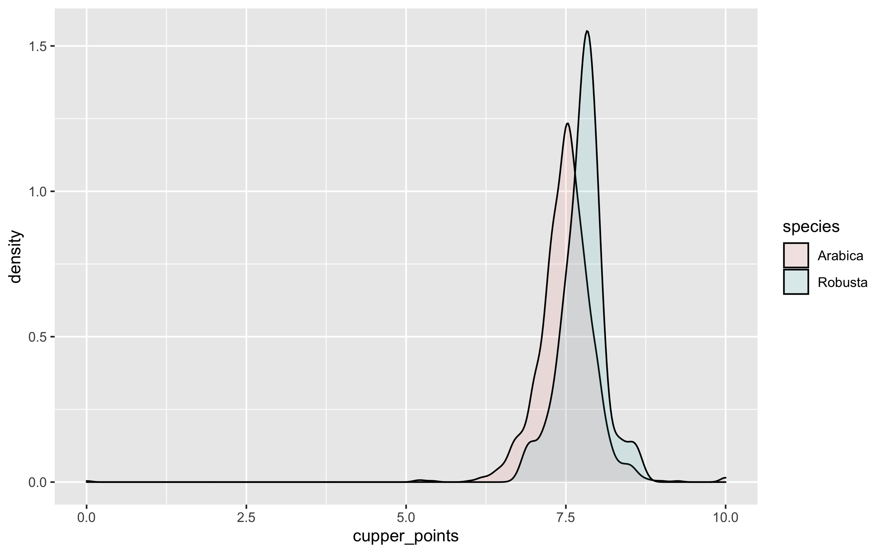
# geom_histogram(position = "identity", alpha = 0.7, show.legend = FALSE)TIDYMODELS
I have never used tidymodels, so let’s see how this goes. Let’s try to tackle the regression model first. From the skim package, we know we have no missing values or junky data for this. Nice!
First thing to do is narrow our data and make it ripe for modeling. TidyTuesday mentions that Yorgos Askalidis already determined that altitude, processing_method and color have no bearing to the cupping score, and I think that makes sense. I will omit those features for now. That leaves us with species, country of origin and several ratings and measurements of the coffee samples. I am going to take the top ten countries only (out of 36 in the data) and lump the rest into “Other” with forcats. This is simply to speed up the processing without losing too much information gain for the feature.
Note - I went back after trying the models a few times and removed ‘species’. In this smaller, filtered dataset there are only 3 records with Robusta coffee beans. It caused me some issues, and with only 3 members of the minority class, I decided to just remove it completely.
coffee <- coffee_ratings %>%
  mutate(id = row_number()) %>% # add ID field, convert NA to Other
  select(id, country_of_origin, variety, aroma:moisture) %>% # select features
  mutate(country_of_origin = case_when(
    country_of_origin %in% top_countries ~ country_of_origin,
    TRUE ~ "Other"
  )) %>%
  mutate_if(is.character, as.factor) %>% # convert country and variety to factors
  filter(cupper_points != 0) %>% # remove 0 point scores as junk data
  drop_na() # drop NA for country and variety fields. only affects 200 records
Split the data
Note - I initially tried to stratify by species, even though there aren’t many Robusta coffee samples in the data. I ended up removing this due to the severe class imbalance. It may have been worth the effort to upsample Robusta and then stratify by species.
set.seed(1234)

coffee_split <- coffee %>%
  initial_split()

coffee_train <- training(coffee_split)
coffee_test <- testing(coffee_split)
Naive linear model with no scaling or pre-processing
lm_spec <- linear_reg() %>%
  set_engine(engine = "lm")

lm_spec
## Linear Regression Model Specification (regression)
##
## Computational engine: lm## Linear Regression Model Specification (regression)
##
## Computational engine: lm
lm_fit <- lm_spec %>%
fit(cupper_points ~ .,
data = coffee_train
)
lm_fit## parsnip model object
##
## Fit time: 10ms
##
## Call:
## stats::lm(formula = formula, data = data)
##
## Coefficients:
## (Intercept)
## 2.501509
## id
## -0.000309
## country_of_originColombia
## -0.099026
## country_of_originCosta Rica
## -0.020488
## country_of_originEthiopia
## 0.029321
## country_of_originGuatemala
## -0.045107
## country_of_originHonduras
## -0.013921
## country_of_originMexico
## 0.030019
## country_of_originOther
## 0.003251
## country_of_originTaiwan
## -0.134839
## country_of_originTanzania, United Republic Of
## 0.052325
## country_of_originUnited States (Hawaii)
## -0.316031
## varietyBlue Mountain
## -0.234205
## varietyBourbon
## -0.004215
## varietyCatimor
## 0.018467
## varietyCatuai
## 0.015110
## varietyCaturra
## 0.036397
## varietyEthiopian Heirlooms
## -0.094942
## varietyEthiopian Yirgacheffe
## 0.011110
## varietyGesha
## 0.046588
## varietyHawaiian Kona
## 0.296594
## varietyJava
## 0.007740
## varietyMandheling
## 0.001044
## varietyMarigojipe
## -0.006565
## varietyMundo Novo
## -0.047911
## varietyOther
## -0.019686
## varietyPacamara
## -0.067598
## varietyPacas
## -0.001151
## varietyPache Comun
## -0.134161
## varietyPeaberry
## -0.022037
## varietyRuiru 11
## -0.016437
## varietySL14
## 0.017365
## varietySL28
## -0.256004
## varietySL34
## -0.055397
## varietySulawesi
## 0.040376
## varietySumatra
## 0.096590
## varietySumatra Lintong
## 0.080224
## varietyTypica
## -0.035801
## varietyYellow Bourbon
## 0.086077
## aroma
## -0.003595
## flavor
## 0.241316
## aftertaste
## 0.278652
## acidity
## 0.040398
## body
## 0.022329
## balance
## 0.194880
## uniformity
## -0.022991
## clean_cup
## 0.013229
## sweetness
## -0.043329
## moisture
## -0.505604library(ranger)
rf_spec <- rand_forest(mode = "regression") %>%
set_engine("ranger")
rf_spec## Random Forest Model Specification (regression)
##
## Computational engine: ranger## Random Forest Model Specification (regression)
##
## Computational engine: ranger
rf_fit <- rf_spec %>%
fit(cupper_points ~ .,
data = coffee_train
)
rf_fit## parsnip model object
##
## Fit time: 468ms
## Ranger result
##
## Call:
## ranger::ranger(formula = formula, data = data, num.threads = 1, verbose = FALSE, seed = sample.int(10^5, 1))
##
## Type: Regression
## Number of trees: 500
## Sample size: 834
## Number of independent variables: 13
## Mtry: 3
## Target node size: 5
## Variable importance mode: none
## Splitrule: variance
## OOB prediction error (MSE): 0.04135314
## R squared (OOB): 0.7374583Both models produce a hefty R squared, > .7! This makes me nervous as it’s likely too good to be true (overfit). I know that I skipped some preprocessing steps just to see how these models worked, so let’s go back and see if some recipes can bring my models back down to earth.
Preprocessing With Recipes
- Let’s create a bland, vanilla recipe to start off
rec_obj <- recipe(cupper_points ~ ., data = coffee_train) %>%
  update_role(id, new_role = "ID") %>%
  step_normalize(all_predictors(), -all_nominal()) %>%
  step_dummy(all_nominal())

summary(rec_obj)
## # A tibble: 14 x 4
## variable type role source
## <chr> <chr> <chr> <chr>
## 1 id numeric ID original
## 2 country_of_origin nominal predictor original
## 3 variety nominal predictor original
## 4 aroma numeric predictor original
## 5 flavor numeric predictor original
## 6 aftertaste numeric predictor original
## 7 acidity numeric predictor original
## 8 body numeric predictor original
## 9 balance numeric predictor original
## 10 uniformity numeric predictor original
## 11 clean_cup numeric predictor original
## 12 sweetness numeric predictor original
## 13 moisture numeric predictor original
## 14 cupper_points numeric outcome originalI tell the recipe not to use the “id” column in the analysis and we can see that it is classified as a “ID” and not “predictor”. I run summary on the recipe object and can see the type of role the variables have, as well as the type. It is important to note that ‘nominal’ is yet another term to describe a factor/string/non-numeric.
Then I use the step_* functions to normalize the data (it centers and scales numerical features) and to create dummy variables for all of my nominal (non-numeric) features.
So we built our recipe. Next step is to prep and juice. I’m getting thirsty.
coff_train <- juice(prep(rec_obj))

dim(coff_train)
## [1] 834 50names(coff_train)## [1] "id"
## [2] "aroma"
## [3] "flavor"
## [4] "aftertaste"
## [5] "acidity"
## [6] "body"
## [7] "balance"
## [8] "uniformity"
## [9] "clean_cup"
## [10] "sweetness"
## [11] "moisture"
## [12] "cupper_points"
## [13] "country_of_origin_Colombia"
## [14] "country_of_origin_Costa.Rica"
## [15] "country_of_origin_Ethiopia"
## [16] "country_of_origin_Guatemala"
## [17] "country_of_origin_Honduras"
## [18] "country_of_origin_Mexico"
## [19] "country_of_origin_Other"
## [20] "country_of_origin_Taiwan"
## [21] "country_of_origin_Tanzania..United.Republic.Of"
## [22] "country_of_origin_United.States..Hawaii."
## [23] "variety_Blue.Mountain"
## [24] "variety_Bourbon"
## [25] "variety_Catimor"
## [26] "variety_Catuai"
## [27] "variety_Caturra"
## [28] "variety_Ethiopian.Heirlooms"
## [29] "variety_Ethiopian.Yirgacheffe"
## [30] "variety_Gesha"
## [31] "variety_Hawaiian.Kona"
## [32] "variety_Java"
## [33] "variety_Mandheling"
## [34] "variety_Marigojipe"
## [35] "variety_Moka.Peaberry"
## [36] "variety_Mundo.Novo"
## [37] "variety_Other"
## [38] "variety_Pacamara"
## [39] "variety_Pacas"
## [40] "variety_Pache.Comun"
## [41] "variety_Peaberry"
## [42] "variety_Ruiru.11"
## [43] "variety_SL14"
## [44] "variety_SL28"
## [45] "variety_SL34"
## [46] "variety_Sulawesi"
## [47] "variety_Sumatra"
## [48] "variety_Sumatra.Lintong"
## [49] "variety_Typica"
## [50] "variety_Yellow.Bourbon"coff_train## # A tibble: 834 x 50
## id aroma flavor aftertaste acidity body balance uniformity clean_cup
## <int> <dbl> <dbl> <dbl> <dbl> <dbl> <dbl> <dbl> <dbl>
## 1 2 3.84 3.55 3.27 3.35 3.35 2.68 0.312 0.225
## 2 3 2.77 3.03 3.04 2.84 3.02 2.68 0.312 0.225
## 3 5 2.22 3.03 2.54 3.10 3.35 2.41 0.312 0.225
## 4 10 1.66 3.27 3.27 3.10 0.575 2.68 0.312 0.225
## 5 12 2.22 2.78 2.30 2.56 2.09 1.94 0.312 0.225
## 6 13 1.66 3.55 2.77 2.84 1.80 1.68 0.312 0.225
## 7 16 1.40 3.03 3.51 2.05 2.42 1.44 0.312 0.225
## 8 19 2.77 2.26 2.03 2.05 1.50 1.44 0.312 0.225
## 9 21 1.40 2.26 2.03 3.10 2.72 1.44 0.312 0.225
## 10 23 1.96 2.26 2.30 1.51 1.17 1.94 0.312 0.225
## # … with 824 more rows, and 41 more variables: sweetness <dbl>, moisture <dbl>,
## # cupper_points <dbl>, country_of_origin_Colombia <dbl>,
## # country_of_origin_Costa.Rica <dbl>, country_of_origin_Ethiopia <dbl>,
## # country_of_origin_Guatemala <dbl>, country_of_origin_Honduras <dbl>,
## # country_of_origin_Mexico <dbl>, country_of_origin_Other <dbl>,
## # country_of_origin_Taiwan <dbl>,
## # country_of_origin_Tanzania..United.Republic.Of <dbl>,
## # country_of_origin_United.States..Hawaii. <dbl>,
## # variety_Blue.Mountain <dbl>, variety_Bourbon <dbl>, variety_Catimor <dbl>,
## # variety_Catuai <dbl>, variety_Caturra <dbl>,
## # variety_Ethiopian.Heirlooms <dbl>, variety_Ethiopian.Yirgacheffe <dbl>,
## # variety_Gesha <dbl>, variety_Hawaiian.Kona <dbl>, variety_Java <dbl>,
## # variety_Mandheling <dbl>, variety_Marigojipe <dbl>,
## # variety_Moka.Peaberry <dbl>, variety_Mundo.Novo <dbl>, variety_Other <dbl>,
## # variety_Pacamara <dbl>, variety_Pacas <dbl>, variety_Pache.Comun <dbl>,
## # variety_Peaberry <dbl>, variety_Ruiru.11 <dbl>, variety_SL14 <dbl>,
## # variety_SL28 <dbl>, variety_SL34 <dbl>, variety_Sulawesi <dbl>,
## # variety_Sumatra <dbl>, variety_Sumatra.Lintong <dbl>, variety_Typica <dbl>,
## # variety_Yellow.Bourbon <dbl>Baking applies the pre-processing steps that were ‘juiced’ above to the test data. This way, the train and test data will have the same pre-processing steps (aka recipe) applied to them. Clever!
coff_test <- rec_obj %>%
  prep() %>%
  bake(coffee_test)
So now we see all our predictors including all the dummy variables that were generated. Neat.
Better, Faster, Stronger
Now we can go back to the linear and random forest regression models used earlier, but now substitute the data with better processing. I think I see why they went with the “recipe” motif! Like baking, I can swap in ingredients without having to start over from scratch.
lm_fit1 <- fit(lm_spec, cupper_points ~ ., coff_train)
glance(lm_fit1$fit)
## # A tibble: 1 x 11
## r.squared adj.r.squared sigma statistic p.value df logLik AIC BIC
## <dbl> <dbl> <dbl> <dbl> <dbl> <int> <dbl> <dbl> <dbl>
## 1 0.751 0.736 0.204 49.4 2.55e-203 49 168. -237. -0.335
## # … with 2 more variables: deviance <dbl>, df.residual <int>tidy(lm_fit1) %>%
arrange(desc(abs(statistic)))## # A tibble: 49 x 5
## term estimate std.error statistic p.value
## <chr> <dbl> <dbl> <dbl> <dbl>
## 1 (Intercept) 7.71 0.109 70.7 0.
## 2 id -0.000309 0.0000479 -6.45 1.99e-10
## 3 aftertaste 0.0944 0.0163 5.79 1.01e- 8
## 4 balance 0.0665 0.0132 5.02 6.39e- 7
## 5 flavor 0.0789 0.0173 4.56 6.07e- 6
## 6 country_of_origin_Taiwan -0.135 0.0462 -2.92 3.63e- 3
## 7 moisture -0.0230 0.00823 -2.79 5.36e- 3
## 8 country_of_origin_Colombia -0.0990 0.0434 -2.28 2.28e- 2
## 9 sweetness -0.0177 0.00819 -2.16 3.09e- 2
## 10 variety_SL28 -0.256 0.119 -2.16 3.14e- 2
## # … with 39 more rowslm_predicted <- augment(lm_fit1$fit, data = coff_train)
select(lm_predicted, id, cupper_points, .fitted:.std.resid)## # A tibble: 834 x 9
## id cupper_points .fitted .se.fit .resid .hat .sigma .cooksd .std.resid
## <int> <dbl> <dbl> <dbl> <dbl> <dbl> <dbl> <dbl> <dbl>
## 1 2 8.58 8.52 0.0749 0.0562 0.135 0.204 2.80e-4 0.297
## 2 3 9.25 8.45 0.0431 0.795 0.0447 0.202 1.52e-2 3.99
## 3 5 8.58 8.39 0.0707 0.187 0.120 0.204 2.67e-3 0.977
## 4 10 8.5 8.49 0.0721 0.00789 0.125 0.204 5.00e-6 0.0414
## 5 12 8.5 8.34 0.0379 0.162 0.0345 0.204 4.75e-4 0.807
## 6 13 8.33 8.43 0.0435 -0.0979 0.0456 0.204 2.36e-4 -0.492
## 7 16 8.17 8.43 0.0443 -0.264 0.0472 0.204 1.78e-3 -1.33
## 8 19 8.42 8.21 0.0570 0.206 0.0783 0.204 1.92e-3 1.05
## 9 21 8.17 8.25 0.0407 -0.0779 0.0398 0.204 1.29e-4 -0.390
## 10 23 8.58 8.24 0.0402 0.344 0.0388 0.204 2.44e-3 1.72
## # … with 824 more rowsggplot(lm_predicted, aes(.fitted, cupper_points)) +
geom_point(alpha = .2) +
ggrepel::geom_label_repel(aes(label = id),
data = filter(lm_predicted, abs(.resid) > 2)) +
labs(title = "Linear Model: Actual vs. Predicted Cupper Points") +
geom_smooth()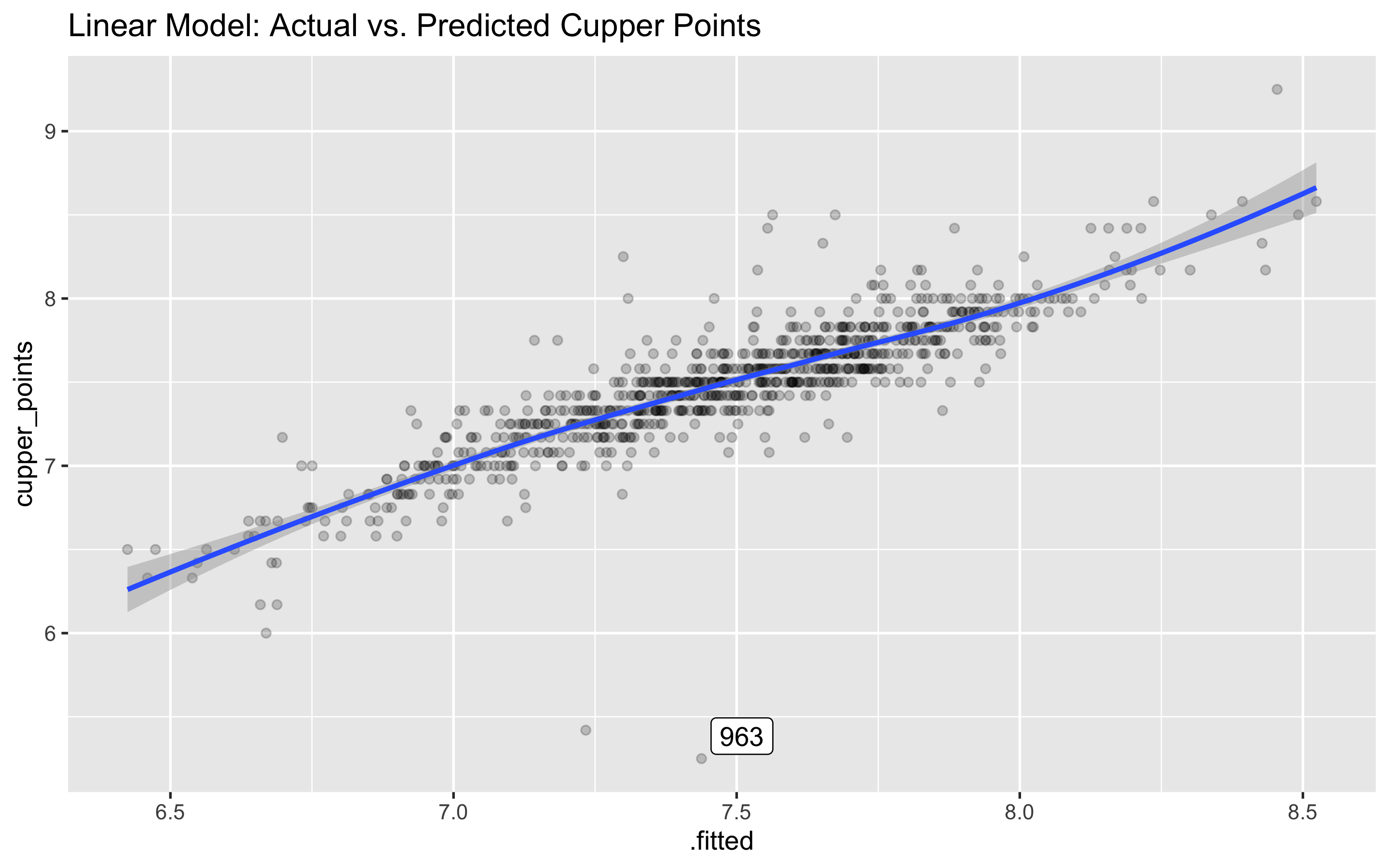
Whoa, what’s up with coffee sample 963? We predicted a score of 7.4 or so, and the real score was a 5.25. This appears just to be a major outlier, so we can likely ignore.
filter(coffee, id == 963)## # A tibble: 1 x 14
## id country_of_orig… variety aroma flavor aftertaste acidity body balance
## <int> <fct> <fct> <dbl> <dbl> <dbl> <dbl> <dbl> <dbl>
## 1 963 Taiwan Typica 7.83 7.75 7.67 7.83 7.83 7.75
## # … with 5 more variables: uniformity <dbl>, clean_cup <dbl>, sweetness <dbl>,
## # cupper_points <dbl>, moisture <dbl>Now let’s repeat for the random forest model. Note - glance does not work for ranger objects like rf_fit1$fit.
rf_fit1 <- fit(rf_spec, cupper_points ~ ., coff_train)
rf_fit1$fit
## Ranger result
##
## Call:
## ranger::ranger(formula = formula, data = data, num.threads = 1, verbose = FALSE, seed = sample.int(10^5, 1))
##
## Type: Regression
## Number of trees: 500
## Sample size: 834
## Number of independent variables: 49
## Mtry: 7
## Target node size: 5
## Variable importance mode: none
## Splitrule: variance
## OOB prediction error (MSE): 0.04222097
## R squared (OOB): 0.7319486rf_predicted <- bind_cols(.fitted = rf_fit1$fit$predictions, data = coff_train)
select(rf_predicted, id, cupper_points, .fitted)## # A tibble: 834 x 3
## id cupper_points .fitted
## <int> <dbl> <dbl>
## 1 2 8.58 8.60
## 2 3 9.25 8.31
## 3 5 8.58 8.54
## 4 10 8.5 8.41
## 5 12 8.5 8.30
## 6 13 8.33 8.36
## 7 16 8.17 8.33
## 8 19 8.42 8.24
## 9 21 8.17 8.29
## 10 23 8.58 8.14
## # … with 824 more rowsggplot(rf_predicted, aes(.fitted, cupper_points)) +
geom_point(alpha = .2) +
# ggrepel::geom_label_repel(aes(label = id),
# data = filter(rf_predicted, abs(.resid) > 2)) +
labs(title = "Random Forest: Actual vs. Predicted Cupper Points") +
geom_smooth()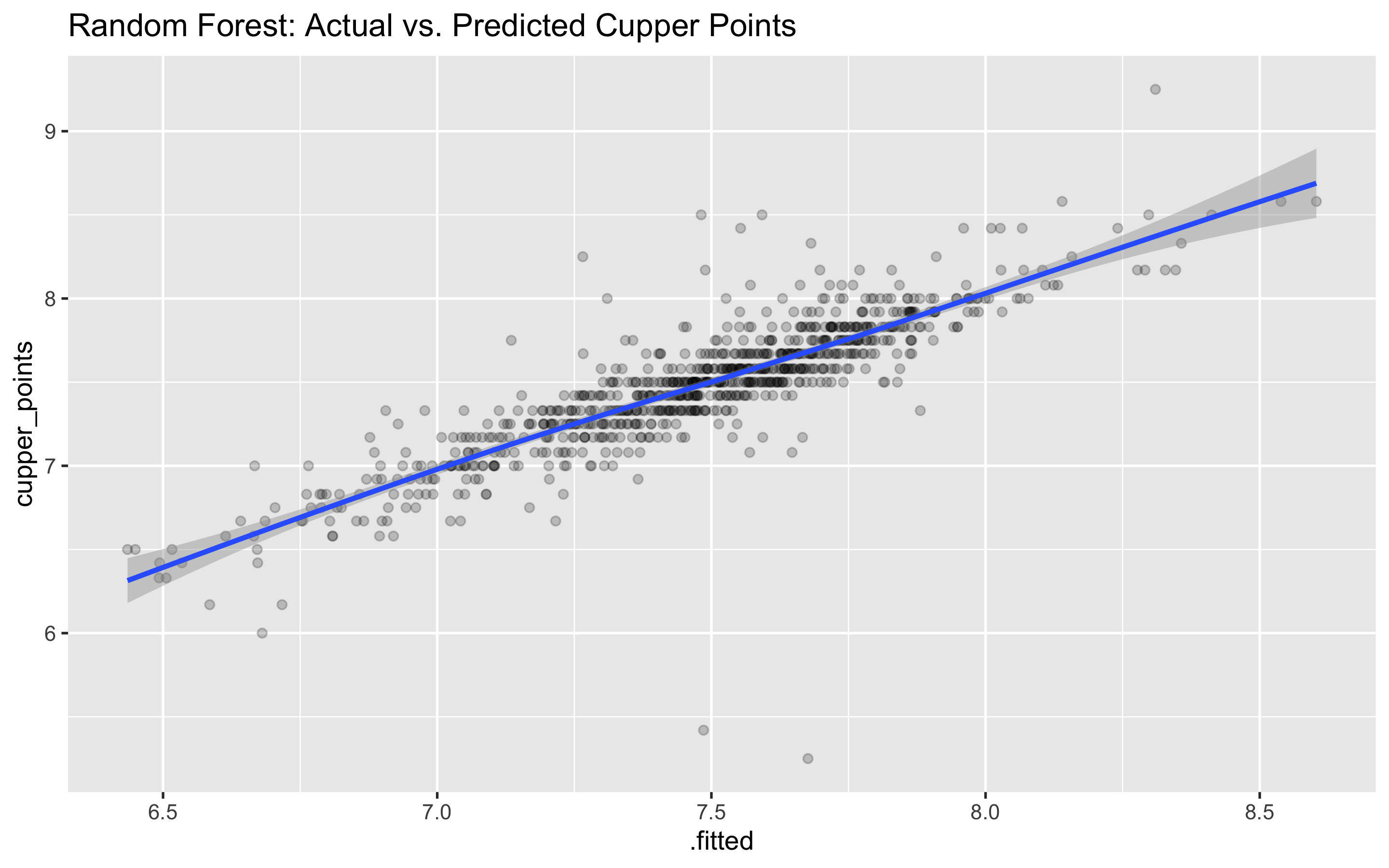
results_train <- lm_fit1 %>%
  predict(new_data = coff_train) %>%
  mutate(
    truth = coff_train$cupper_points,
    model = "lm"
  ) %>%
bind_rows(rf_fit1 %>%
    predict(new_data = coff_train) %>%
    mutate(
      truth = coff_train$cupper_points,
      model = "rf"
    ))
results_train %>%
group_by(model) %>%
rmse(truth = truth, estimate = .pred)## # A tibble: 2 x 4
## model .metric .estimator .estimate
## <chr> <chr> <chr> <dbl>
## 1 lm rmse standard 0.198
## 2 rf rmse standard 0.114Apply model to the test set
lm_fit1 %>%
  predict(coff_test) %>%
  bind_cols(coff_test) %>%
  metrics(truth = cupper_points,
          estimate = .pred) %>%
  bind_cols(model = "lm") %>%
  bind_rows(
    rf_fit1 %>%
      predict(coff_test) %>%
      bind_cols(coff_test) %>%
      metrics(truth = cupper_points,
        estimate = .pred
      ) %>%
  bind_cols(model = "rf")
  )
## # A tibble: 6 x 4
## .metric .estimator .estimate model
## <chr> <chr> <dbl> <chr>
## 1 rmse standard 0.244 lm
## 2 rsq standard 0.629 lm
## 3 mae standard 0.144 lm
## 4 rmse standard 0.231 rf
## 5 rsq standard 0.664 rf
## 6 mae standard 0.130 rfWe see that the random forest and linear model are both very close together in performance. However, the random forest does have a small RMSE and higher R squared, which means it does a slightly better job explaining the variance and has less overall error in predicting the ratings.
Next Steps
I did all of this analysis without knowing anything about tidymodels. Additionally, I am fairly new to using R for predicting values as well. It would be interesting to see how these models perform with cross-validation, optimized parameters and better feature selection.
The concept of a “recipe” which you can modify and reuse is incredibly interesting in this context. I have a lot more to learn here, and would direct readers to the great YouTube videos made by Julia Silge.